Bayesian Probability#
When you’ve learned about probability before, it probably looked something like what we covered last week. In that framework, the probability of an event is defined as
where \(n_S\) represents the total number of “successess” (i.e. trials on which the event took place) out of the total \(n\) trials.This is a useful way to definite probability. It fits a lot of our intuitions—a fair coin has a 50% probability of landing heads up because, if we flip the coin many times, we expect it to land heads half the time. This version of probability is called frequentist probability.
But that’s not the only way to understand probability. Instead, we could say that the percentage 50% represents something about our beliefs about the coin—namely that, if we flip it, it is equally likely to land heads or tails. This approach is called Bayesian probability. There’s a really important distinction here; whereas frequentist probabilities adhere to the long-run frequency of an event after many, many trials, Bayesian probabilities describe our beliefs about what a single trial will be like.
This may not seem to be a very big distinction. But as we shall see, thinking of probability as belief has some major mathematical implications. And while Bayesian probability does present some challenges—pinning down beliefs mathematically can be tricky—it can also be a useful framework for analyzing certain problems. And it turns out to be a really successful model for lots of human, and animal, behavior.
Learning Goals
By the end of this week, you should be able to:
Compare and contrast the Bayesian and frequentist approaches to statistics and identify situations in which each approach might be more advantageous
Apply Bayes’s rule in order to find the maximum a posteriori estimate of both discrete and continuous variables
Describe the mathematical challenges in applying the Bayesian framework to continuous probabilities as well as multiple ways of meeting those challenges
Use the technique of conjugate priors to solve for the full posterior distribution of a parameter, given a likelihood distribution
The Bayesian Approach#
Let’s say we are flipping a coin. We might assume, from the get-go, that this coin is fair, i.e., that it has a 50% probability of landing heads. In frequentist language, we can call the assumption that the coin is fair our null hypothesis. But then we flip the coin several times, and it keeps coming up heads. How many times would it need to come up heads in a row to convince us that it isn’t a fair coin?
In conventional statistics, we always operate with a null hypothesis \(H_0\) (the coin is fair) and an alternative hypothesis \(H_A\) (the coin isn’t fair). To reject the null, we need to show that the probability of data as extreme as or more extreme than our data occuring if the null hypothesis is true (that is, our \(p\)-value) is below some threshold (our chosen significance level).
Let’s say, then, that we choose a significance level \(\alpha = 0.05.\) How many times will our coin need to show up heads for us to be convinced that it is unfair? We need to figure out the odds of getting a sequence of heads of a given length under our null hypothesis that the coin is fair. This isn’t too tricky:
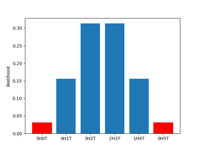
So the odds of 5 heads are below 0.05. Is that our answer? Not quite; remember, we have to take into account all possibilities that are as extreme as (or more extreme than) our data. While there’s nothing more extreme than our data under this null distribution (which is a binomial distribution), there is one possibility as extreme—5 tails. So the \(p\)-value for 5 heads under a \(H_0\) of a fair coin and a \(H_A\) of an unfair coin is \(0.03125 + 0.03125 = 0.0625.\) (You can see what that looks like in the diagram below.) That’s a bit above our significance level. So we need to see 6 heads in a row to reject our null hypothesis and conclude that the coin is unfair.
Under certain circumstances, this may make sense. But in the world we live in, we expect that almost all coins are fair. If you flipped a random coin you found in your pocket 6 times and got heads every time, you probably would not conclude that there was something wrong with that coin. A frequentist framework can’t accommodate this intuition. But a Bayesian framework can.
Applying Bayes’s Rule#
The first step in using the Bayesian framework here is making mathematically concrete what we mean by “almost all coins are fair.” Let’s say it’s a fact that only 1 out of every 10000 coins is unfair, and the rest are all fair—and, furthermore, that every unfair coin lands heads 90% of the time and tails 10% of the time. So if someone gives us a random coin, before flipping that coin, we should think the odds of that coin being fair are 99.99%. This is called our prior—it describes our beliefs prior to making any observations. In Bayesian statistics, we always, always have a prior, and we need to be able to state it mathematically.
Definition
In Bayesian statistics, the prior is a probability distribution describing your beliefs about the outcome of a probabilistic process before observing that process.
Before flipping the coin, then, this is our information:
What happens once we have flipped the coin? We now have a new piece of information. As we did in the frequentist framework, we can calcuate the conditional probability that the coin would have landed heads 6 times in a row, given the assumption that it was fair. This probability is about 1.56%. So we have:
We’ve seen this sort of expression before—it’s just the likelihood of our data! Part of the reason we spent so muh time talking about likelihood last week is that you have to understand likelihood to understand the Bayesian framework.
Previously, we calculated multiple likelihoods for our data and compared them to decide what we thought was going on in our experiment—comparing the likelihoods of different patterns of neural activity in light vs. dark conditions, for example. In this case, that would looke like calculating both \(p(\text{evidence} | \text{fair})\) and \(p(\text{evidence} | \text{unfair})\) and seeing which was higher. And that’s a totally valid approach for solving many problems. But it doesn’t allow us to incorporate our prior belief that the coin is very likely to be fair.
To do that, we want to calculate not \(p(\text{evidence} | \text{fair})\), but rather \(p(\text{fair} | \text{evidence}).\) Fortunately, we have a formula that tells us exactly how to find that, given what we know: Bayes’s rule.
Bayes’s Rule
If you know \(p(A|B)\), it’s straightforward to calculate \(p(B|A)\):
Before we use Bayes’s rule, let’s break it down a little bit. As we’ve mentioned, \(p(B)\) is our prior, and it describes our belief about the probability of \(B\) before taking our newly observed evidence to account. \(p(A|B)\) is the likelihood of our evidence, assuming that the prior is true. And, in analogy to the term “prior,” \(p(B|A)\) is our posterior—our belief about the odds of \(B\) after taking the evidence into account. (We’ll discuss \(p(A)\) in more detail in a bit; it’s called the normalization constant, for reasons that will become clear.)
Definition
In Bayesian statistics, the posterior is a probability distribution describing your beliefs about the outcome of a probabilistic process after observing that process. It is proportional to the product of the prior and the likelihood.
It’s not too difficult to derive Bayes’s rule from some other facts about probability. Recall that the joint probability of two events, \(p(A,B)\)—say, the chance that it’s a summer day (\(A\)) and the temperature is above 80\(^{\circ}\) (\(B\))—is just the probability of the first event times the probability of the second event given the first event: \(p(B|A)p(A).\)
So, the chance that it’s a summer day and the temperature is above 80\(^{\circ}\) is just the probability it’s a summer day, \(p(A) = 0.25\), times the probability that the temperature is above 80\(^{\circ}\) given that it’s a summer day, \(p(B|A) = 0.2,\) or \(p(B|A)p(A) = 0.05.\) We could also find this answer by multiplying the probability the temperature is above 80\(^{\circ}\), \(p(B) = 0.05,\) times the probability it’s a summer day given that the temperature is above 80\(^{\circ}\), \(p(A|B) = 1,\) to get the same joint probability, \(p(A|B)p(B) = 0.05.\)
So we have for any two events, \(A\) and \(B\),
or, in plain English, the posterior probability is the prior times the likelihood, divided by the normalization constant.
To use Bayes’s rule for our fair coin example, we plug in “evidence” for \(A\) and “fair” for \(B,\) and this is what we get:
We already have both terms in the numerator, our prior and our likelihood. But what we don’t have is the normalization constant, which is the total probability of our evidence—the odds of getting 6 heads in a row if we don’t know ahead of time whether the coin is fair or unfair.
Fortunately, for this problem, that probability isn’t too hard to calculate. It’s analogous to the problem of finding the overall odds that the temperature will be above 80\(^{\circ}\) on any random day if we only know the odds it will be above 80\(^{\circ}\) given that it’s a summer day (\(p(\text{hot}|\text{summer}) = 0.2\)) and the odds it will be above 80\(^{\circ}\) given that it’s not a summer day (\(p(\text{hot}|\text{not summer}) = 0\)). All we have to do here is calculate the odds that it’s a hot day and it’s summer, the odds that it’s a hot day and it’s not summer, and add the two together:
This is an implementation of the “law of total probability,” which states that, if we have a set of events \(B_1, B_2, B_3, \dots, B_n\) that are all mutually exclusive but also have probabilities that add to 1—that is, one of them must be true—then we can find the probability of any other event \(p(A)\) by adding \(p(A,B_1) + p(A,B_2) + \dots + p(A,B_n).\) It’s worth noting that we can’t in general add the probabilities of two events together to find the probability of either event occurring, as we did here when we found a probably of a hot day by adding the probability of a hot summer day to the probability of a hot non-summer day. But we can do that if the two events are mutually exclusive—if they can never happen at the same time. Since a summer day is definitionally not a non-summer day, we’re safe doing that in this case.
We can take the same approach when it comes to fair and unfair coins:
The first term in the sum is just our numerator—great! But to find the second term we need to calculate two new probabilities, \(p(\text{evidence}|\text{unfair})\) and \(p(\text{unfair})\). We get \(p(\text{unfair})\) from the facts about the number of fair and unfair coins (one out of every 10000 coins is unfair), and \(p(\text{evidence}|\text{unfair})\) from our facts about how unfair coins work (they come up heads 90% of the time). So we can say:
We finally have all the information we need!
So even after seeing the coin come up heads 6 times in a row, we should still think it’s about 97% likely that the coin is fair. This is far different from what the frequentist framework suggested, and it should accord a bit more with our intuitions about what the world is like. If you took a random quarter out of your wallet, flipped it 6 times, and got heads every time, you probably wouldn’t conclude that the coin is unfair! That’s because you have a prior belief that a random coin is very, very likely to be fair.
That’s the power of the Bayesian framework—unlike the frequentist framework, it can accommodate our baseline, or prior, beliefs about the world.
Bayesian Updating and Bayesian Priors#
The Bayesian framework has another secret power. Let’s say we flip the coin three more times and it comes up heads again every time. We want to update our belief that the coin is fair, based on this new evidence. What does that look like? Let’s put Bayes’s rule to work:
But where do we include the 6 heads that we have already observed into this equation? The trick is to encode it in our prior probability, \(p(\text{fair}).\) In fact, all we have to do is take our previous posterior probability, the probability that our coin is fair given our observation of 6 heads, and plug it in here as our prior.
This should make some logical sense. After observing the 6 heads, we updated our belief that the coin is fair. So that new belief becomes our prior belief before making any additional observations. The posterior we obtain after observing some past evidence becomes our prior for observing any future evidence.
So let’s plug in our numbers and see how the math works out. Remember, our prior \(p(\text{fair})\) (as well as \(p(\text{unfair})\)) will come from the calculation we did above, where we found a posterior probability of 0.967 that the coin was fair. The odds of 3 heads if the coin is fair are just \(0.5^3 = 0.125\); the odds if the coin is unfair are \(0.9^3 = 0.729.\)
With three additional observations, we now have a posterior belief of 83.4% that the coin is fair. If we continue to observe heads (and make this posterior into a new prior in order to update our belief), the odds of the coin being fair will continue to fall. Eventually, if we observe enough heads, the extremely low likelihood of observing that evidence under the assumption that the coin is fair will overwhelm our prior, which was biased strongly toward the coin being fair.
But what happens when we don’t have much evidence—when we’ve only made something like 6 observations? In such cases, the prior remains extremely powerful. With a prior of 99.99% odds that the coin was fair, our posterior belief in the coin being fair was still high after 6 observations—96.7%. But what if we start with a different prior? What if we have a roommate who is a magician and uses trick coins, so we think the odds of our coin being fair are only, say, 80%? Let’s apply Bayes’s rule to our original scenario of observing 6 heads with this new prior:
With this new prior, after observing the 6 heads, we will think there’s only about a 10% chance that the coin is fair. This makes sense—if it’s more likely the coin is unfair in the first place, then the observation of 6 heads will seem much more convincing! But it also highlights how essential an accurate prior is to the successful application of the Bayesian framework.
When we are undertaking a Bayesian update, as we did above after the observation of 3 new head flips, the question of the prior is trivial—it’s just our previous posterior. But to get started we needed to stipulate our prior, that only 1 of every 10,000 coins is unfair. If we were incorrect in that assumption—if in fact 2 of every 10 coins were unfair—then we would have been very, very wrong to conclude that the coin was likely fair. Inaccurate priors lead to inaccurate conclusions.
In the real world, defining a prior is often more an art than a science. There are a number of strategies out there for defining priors and ensuring that priors are reasonable, though they are outside of the scope of this course. But it is essential to remember just how important priors are to our final result.
One coda, however—let’s check what happens when we have lots and lots of evidence. Let’s say we see 30 heads in a row. What will our posterior belief be, with a prior belief of 99.99% that the coin was fair?
So at this point we’ll believe it’s nearly impossible that the coin is fair. What if we had a different prior–say, a 50/50 chance of being fair or unfair?
Yes, this probability is smaller; but both numbers are so small that the difference is pretty much negligible. What this exercise demonstrates is that, as we observe more and more data, our prior starts to matter less and less. Eventually, with really extensive evidence, our prior won’t matter at all. But in many situations in science, and many situations in day-to-day reasoning, we don’t have such an overwhelming amount of evidence. In general, priors matter a lot, and the apparent subjectivity of priors is one reason the Bayesian approach receives criticism from people in the frequentist camp.
From Discrete to Continuous#
Now that we know our way around priors, posteriors, and likelihoods, we can start dealing with problems that are a bit more complex. So far, we have focused on a problem that involved just two probabilities—the odds that the coin was fair, and the odds that it was unfair. Often, however, we care about the probabilities of an infinite number of possibilities—every possible height that a person might have, for example—and we capture those probabilities in a probability distribution, like the normal distribution.
Now, as you might expect, using distributions instead of discrete probabilities makes some things a bit more complicated. But Bayes’s rule still applies; we just have to write it a bit differently.
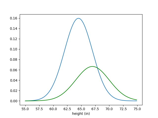
Let’s say that we are interested in figuring out someone’s height. If we know ahead of time that this person is an American cis woman, we might have a prior over the potential values of her height that looks like this:
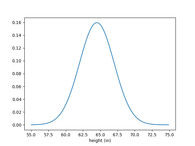
This is just a normal probability density function with a mean of 64.5 and a standard deviation of 2.5. It’s a reasonable prior because it accurately describes what we would observe if we measured the heights of a large number of American cis women—and we don’t know anything else about this woman yet.
But now let’s say we find out that this woman wears size 9 shoes. This is a new piece of evidence, and to incorporate this evidence we need to formulate a likelihood function—a function that describes the chances of an American cis woman of a given height wearing a size 9 shoe. Let’s say that function looks like this:
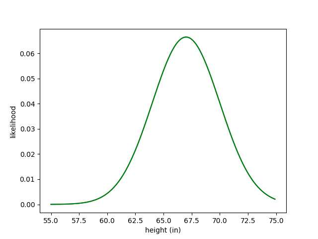
I want to point out something really important here. While our prior is a probability distribution, as it must be—it makes no sense for our beliefs about someone’s height, integrated over all their possible heights, not to equal 1—the likelihood function is not a probability distribution. If, for example, we were to plot the likelihood that Earth’s atmosphere is mostly nitrogen conditioned on the height of this woman, that distribution would integrate to infinity—because that probability is always 1. That’s why our likelihood function here looks quite a bit shorter than our prior; it doesn’t integrate 1. We can see this in our above coin example as well—the likelihood of 6 heads for a fair coin is 0.0156, and for an unfair coin is 0.531, and these do not sum to 1. As we shall soon see, the overall height of our likelihood function doesn’t actually matter; we can multiply it by any constant and still get the same result.
Okay, so what do we do with these two distributions to find our posterior? Let’s look at the prior and likelihood on the same set of axes and try to logically infer what the posterior should look like:
One thing we can probably infer is what the mean of our new distribution should be. If our prior mean is 64.5, and our likelihood mean is 67, then the mean of our posterior should probably be between those two values; our likelihood should drag the prior mean up a bit. Let’s check if our guess is correct:
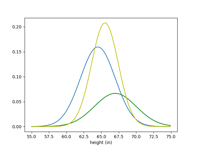
The posterior is shown in yellow. Our guess about the mean looks right! Also notice that the posterior has less variance than either the prior or the likelihood. This should make sense—the more information we get about our parameter of interest (height), the less variance our beliefs about it should have.
So, what is this woman’s height? We don’t have a concrete answer here; just a distribution. But there are ways to get a specific guess for a parameter from a posterior distribution. The most common of these approaches is called maximum a posteriori, or MAP. All MAP involves is taking the value of our parameter associated with the highest probability—the peak of our posterior distribution. In this case, our MAP guess would be about 65.5 inches.
Definition
The maximum a posteriori estimate (MAP) of a random variable is simply the mode of its posterior distribution, or the value of that random variable at which the posterior reaches its peak value.
That’s not the only way that we could have estimated the woman’s height, however. Last week, when we tried to estimate stimulus values based off of neural activity, we looked for the stimulus value that maximized the likelihood of our data. We could in principle do the same thing here—ignore the prior and maximize our likelihood.
Definition
The maximum likelihood estimate (MLE) of a random varialbe is the mode of its likelihood distribution, or the value of that random variable at which the likelihood reaches its peak value.
In general, it’s important to have the right intuitions about how posteriors should look given a particular prior and likelihood. Broadly speaking, the important intuitions are:
The mean of the posterior should be between the mean of the prior and the mean of the likelihood
The mean should end up nearer to the mean of the distribution with the lower variance (because that distribution is more informative)
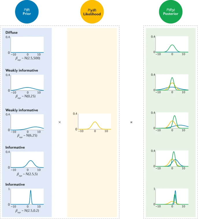
The variance of the posterior should be less than the variances of the prior and the likelihood These intuitions are rules of thumb—they do not always work, though they do work for normal distributions. But in general, they should guide you toward valid Bayesian conclusions and help you check your work. You should be able to guess the right column of the below diagram from the left column. (This diagram is also a great representation of the extent to which proper prior choice matters.)
But intuition isn’t going to get us all of the way there. What we need to know is how to solve for the posterior mathematically.
Bayes’s Rule for Continuous Distributions#
Last week, we discussed how to calculate a likelihood \(p(y | \theta)\)—by calculating the probability density function’s values at each of our observations as a function of \(\theta\), and then multiplying all those functions. And for now, we will assume our prior has been given to us. But how to we combine those pieces of information to get our posterior?
Fortunately, we can do for distributions what we did for discrete probabilities. If \(p(\theta)\) describes our prior probability density function over our parameter of interest, \(\theta\), (height in the above example), and \(y\) is our evidence, we can say
Let’s walk through this step-by-step. This is really just our old friend Bayes’s rule. For distributions, what this means is that the posterior distribution over \(\theta\) given some evidence is the same as the product between the prior distribution of \(\theta\) and the likelihood function of the evidence \(y\), divided by some number. (Yes, \(p(y)\) is a number, not a distribution—it just describes the probability of having received the specific evidence that we did in fact receive.)
So to find our posterior, we literally just multiply our prior distribution and our likelihood function. This might sound pretty simple, and it often is. For example, let’s say \(p(\theta)\) and \(p(y|\theta)\) are both normally distributed, as in the height example above:
We still have to normalize this expression, but that’s easy, since we know how to normalize a normal distribution—we know what the coefficient in front of any normal is \(\frac{1}{\sqrt{2\pi}\sigma}\). So we don’t even have to worry about \(p(y)\) at all.
Often, though, we do have to worry about \(p(y),\) and that poses problems. To find the total probability of the evidence in the coin example from way at the beginning, we had to add the joint probability of the evidence with each possible condition (the coin is fair, or the coin is unfair). That was fine when we only had two possibilities to worry about. But now, when we aren’t worried about whether a coin is fair or unfair but about what its bias is over a continuous range of values, we have an infinite number of possible conditions. That means we can’t add. We have to integrate.
That Pesky Normalization Constant#
So what is this normalization constant that we are trying to deal with? Remember, if we have just two possible conditions, \(c_1\) and \(c_2,\) finding \(p(y)\) is easy:
This is doable for any finite number of conditions. But it isn’t if we have an infinite number of possible values for \(\theta\), our parameter of interest. In such a situation, we have to integrate:
As we’ve mentioned before, this value, \(p(y),\) is called the normalization constant. We can now see why. The reason we can’t just say that our posterior is equal to \(p(y|\theta)p(\theta),\) or our likelihood times our prior, is that our posterior distribution must be a valid probability density function, and all probability density functions must integrate to 1. But we have no guarantee that this product \(p(y|\theta)p(\theta)\) integrates to 1. So we have to integrate over the entire product \(p(y|\theta)p(\theta)\) to get the current area under our curve and then divide by the result, to confirm that the area under our posterior distribution will in fact be 1. That’s why \(p(y)\) is called our normalization constant—it makes sure that our posterior is normalized.
Often, we simply cannot calculate this integral, which means that there is no analytic way to solve for our posterior. But \(p(y)\) is a constant, so we can at least say
So we can figure out the shape of \(p(\theta | y),\) which lets us know which \(\theta\) are more or less likely. We can even find the MAP estimate of \(\theta,\) because that’s just the value of \(\theta\) where our posterior distribution reaches its peak. But without that normalization constant, we can’t fully solve for our posterior distribution. And that can be a major limitation. In fact, the difficulty of calculating these integrals is part of the reason that the Bayesian framework remained unpopular for so long.
Fortunately, there are a number of techniques we can use to overcome this hurdle. Some of these techniques require computer simulation and numerical analysis. But occassionally we can find a closed-form solution for our posterior distribution, using the method of conjugate priors.
Conjugate Priors#
In some cases, we can solve for \(p(\theta | y)\) analytically. These are cases where we know how to normalize the functional form of \(p(\theta | y)\). In the case of height above, where I assumed that our prior and our likelihood were both known normal distributions, we were able to solve for our posterior because the product of two normal distributions is also a normal distribution, and it’s easy to normalize a normal distribution—just include that \(\frac{1}{\sqrt{2\pi}\sigma}\) in front. In general, if multiplying our prior and our likelihood gives us a known distribution (like a normal distribution), we are safe; we can normalize those distributions easily.
This means that there are pairs of priors and likelihoods that will give us easily manageable posteriors. We don’t get to choose our likelihood, but we do get to choose our prior. And as it turns out, for certain likelihoods, there exist families of priors called conjugate priors that make our lives really, really easy. As we saw above, the conjugate prior of a normal is a normal.
Definition
A conjugate prior for a given likelihood distribution is a prior that, when multiplied by the likelihood, yields a posterior that is from the same family of distributions as the prior.
Let’s run through a full Bayesian inference problem using conjugate priors. We’ll use the same coin example from the beginning, but we’ll make it a bit more realistic—by allowing the coin’s bias, \(\theta\), to range continuously from 0 to 1. Let’s say we flip the coin \(n\) times and get \(y\) heads. What’s the likelihood? Well, this is just a classic binomial distribution problem:
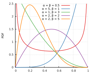
In theory, our prior over the coin’s bias could be anything. But if we want our Bayesian inferece to work out nicely, we have to pick a specific sort of distribution to represent our prior—in this case, the beta distribution. The probability density function for the beta distribution is:
As you can see, the beta distribution is very closely related to the binomial distribution. And we can choose whatever \(\alpha\) and \(\beta\) we want for the beta distribution, which comes in super handy; it allows us to give our prior a ton of different shapes, while still keeping it beta. (As a note—\(\alpha\) and \(\beta\) don’t actually have to be integers, but the coefficient is easier to write if they are.)
So, let’s do some inference. Let’s say we think our coin is fair to start off, and we’re pretty confident in that assumption. So we want a distribution with a quite strong peak at 0.5. We can achieve this by setting \(\alpha = \beta\) and having them both take fairly high values. Let’s see what our prior looks like of both are 20:
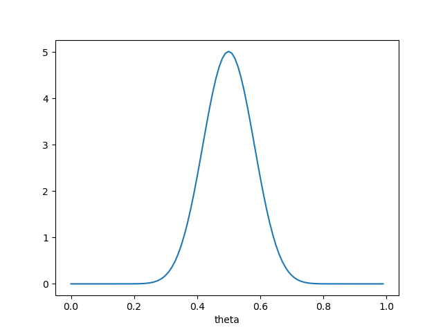
So the functional form of our prior is
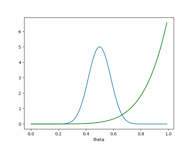
Now let’s say we end up flipping our coin and getting 6 heads. So \(n\) is 6 and \(y\) is 6, which means our likelihood is:
because there is only one way to choose 6 items from a set of 6! This is what our prior and likelihood look like on the same axes:
Now we can find our posterior. We write:
This is not normalized. But it is proportional to a beta distribution with \(\alpha = 26\) and \(\beta = 20\)—and we know how to normalize that! So we have
We didn’t even have to deal with \(p(y)\) because we already knew what we needed to do to normalize our posterior. Plotting the prior, likelihood, and posterior on the same axes, we get the following:
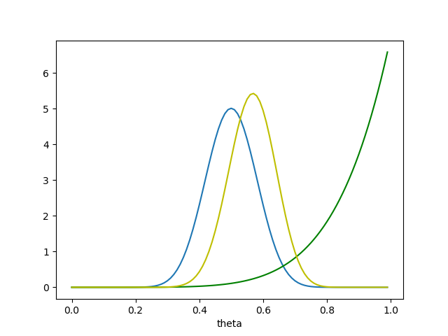
So our beliefs about the coin have shifted a bit to the right! After all those tails, our MAP is that the coin has about a 55% chance of landing heads. But there’s still plenty of probability mass at \(\theta = 0.5\)—it’s definitely still very possible that the coin is fair. If we had started with a much stronger prior—say, \(\alpha = \beta = 100\)—we would have seen something different:
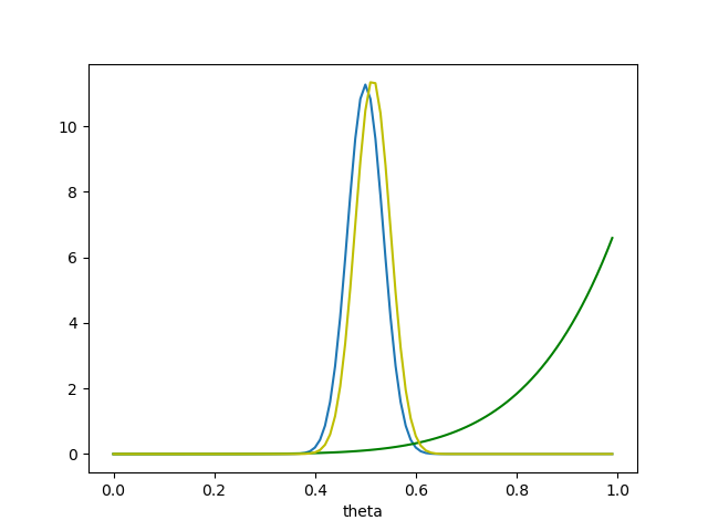
We would have remained quite confident that the coin was fair, or very close to it.
This is the power of conjugate priors—they make Bayesian inference easy. We can’t choose what our likelihood looks like, but we can choose our prior; and even when we restrict ourselves to a conjugate family, there are still tons of possibilities for what a prior might look like.
Of course, depending on what the likelihood is like, conjugate priors are not always an option. That’s when we have to use numerical methods—basically, brute-forcing the problem with a computer—to solve for the posterior.