Probability#
It’s impossible to do experimental science without understanding probability. No matter what field you are in, probability permeates every aspect of the scientific process. Hypotheses often ask not whether changing a certain condition makes a particular outcome happen, but whether it makes that outcome more or less likely. And when we analyze data, we often ask: What’s the probability that I would have obtained this result, if my hypothesis were not true?
Part of why we cover probability in this class is because neuroscience is an experimental science. But probability is also fundamental to how we understand the brain. We often talk about neurons like they are deterministic machines — as if a neuron that responds to a particular stimulus will always fire, and fire in exactly the same way, when the animal perceives that stimulus. But biology doesn’t work that way. Biology is random, and finicky — proteins flip-flop from one conformation to another, neurotransmitters drift across synapses, and ions careen about the cell. All of this means that there’s a high degree of randomness in how neurons behave. We use the tools of probability to get a handle on that randomness — to model how neurons work, to understand the role they play in behavior, and to figure out what their activity patterns mean.
Learning Goals
By the end of this week, you should be able to:
Apply the concepts and principles of basic probability theory — like events, sample spaces, independence, mutual exclusivity, and conditional probability — to calculate the probabilities of specified events
Use random variables to describe probabilistic events, and calculate the expected value and variance of those variables
Choose and deploy common probability distributions — like Bernoulli, Poisson, and Gaussian — to model neuroscientific phenomena
Calculate the likelihood function for a given model and use it to fit that model to data
Basic Probability Theory#
Events and Sample Spaces#
What does it mean to say “There’s a 50% chance of rain tomorrow”? There are actually a few different answers to this question, and next week we will focus on one that you might not have thought of before. But this week, we’ll be taking the conventional approach to this question, which goes something like this: If you take the set of all possible days that we could have tomorrow, you’ll find that half of them are rainy.
The idea of the “set of all possible days,” or more generally the set of possibilities, is a really important one in probability. Formally speaking, it’s referred to as the sample space. By leveraging the idea of the sample space, we can work to keep our probability calculations concrete and grounded. Probability gets hard when you lose track of all the possible outcomes; if you work hard to keep them in mind, things get easier.
Definition
A sample space is the set of all of the possible outcomes of some random process — like the weather, or a scientific experiment.
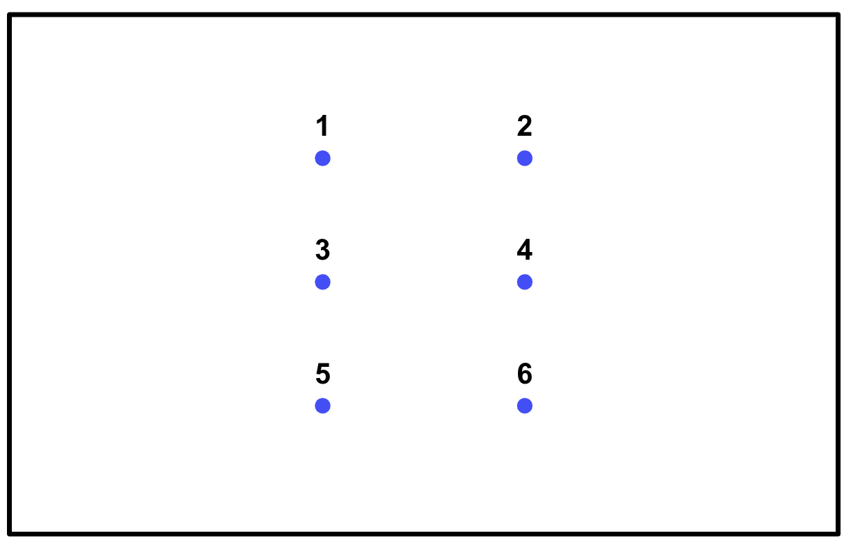
One incredibly simple sample space characterizes all of the possible outcomes of rolling a 6-sided die:
To make use of a sample space, we need to identify the portion of the sample space that we are interested in. In the weather case, it’s those next-day weather patterns that include rain. We call a portion of the sample space an event. This usage is generally pretty intuitive — speaking of “rain tomorrow” as an event makes sense in conventional English — but it’s good to keep the formal definition in mind as well.
Definition
An event is a subset of a sample space.
Let’s bring things back to neuroscience. You are running an experiment on mice, and part of your goal is to characterize sniffing behavior. The sense of smell is really important to mice: the whole front chunk of the mouse brain is devoted to processing smell information. So understanding this sniffing behavior could help you get a better grasp on how mice interact with and understand their environments.
To start, you have a super simple question. Each trial of your experiment involves observing a mouse for 5 seconds. Your question is, how likely is the mouse to sniff on any trial?
Exercise
What’s the sample space here? What’s the event that we are interested in?
Solution
Our sample space is just the set of all possible behavioral patterns that the mouse could engage in in that 5-second trial. The event is the subset of those behaviors that include sniffing.
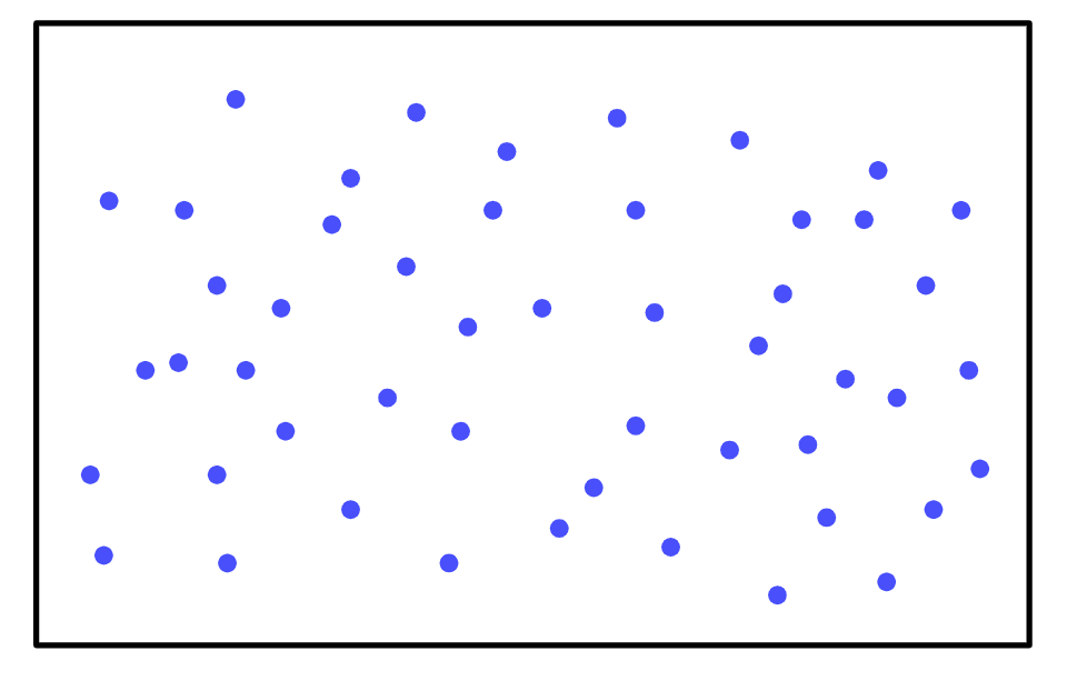
So let’s build our sample space:
To find the probability of the mouse sniffing, all you have to do is count all of the behavioral patterns that include sniffing (shown in red):
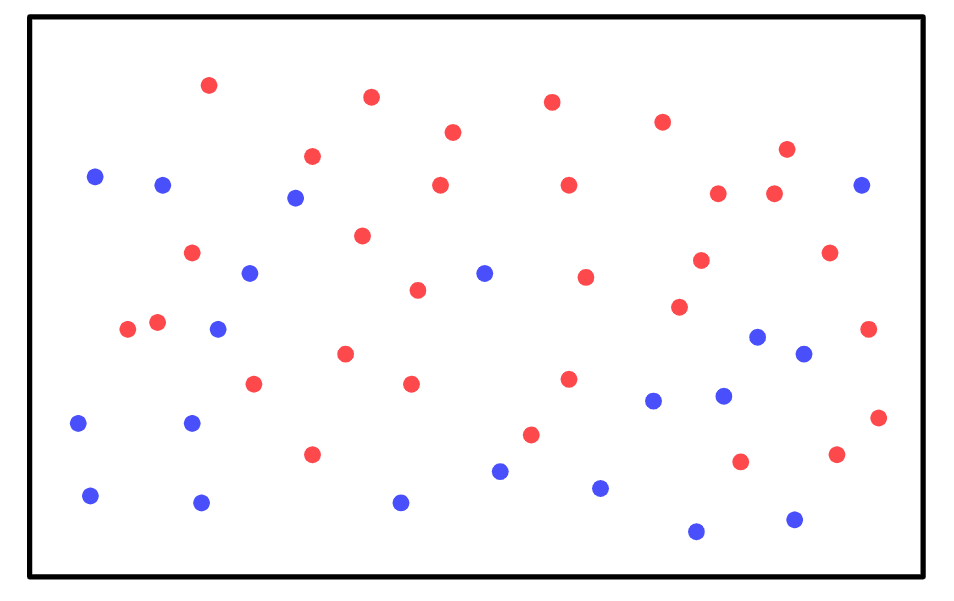
There are 50 behaviors total in the sample space, and 30 of them include sniffing, so the probability of the mouse sniffing in the next trial is 0.6.
I’ve been glossing over a really important detail, however. We defined the sample space as the set of all possible outcomes — how can we possibly enumerate all of the possible behaviors a mouse might engage in in 5 seconds? Strictly speaking, the sample space is infinite. We could never count up all those possibilities.
There are a couple of approaches to managing this problem. The first is to partition the sample space in a reasonable way: to consider not specific outcomes, but rather well-chosen sets of outcomes, as the elements of the sample space. The second is to approximate the sample space by running your experiment repeatedly and collecting the results — or by looking at the results that the same random process has produced in the past.
Let’s start with partitioning. What does this look like in practice? First, there’s one important constraint here — if we want to be able to count up the elements in our event, and then find the probability of the event by dividing that number by the size of our sample space, then all of the elements in the sample space need to be equally likely. (You could also create a sample space with elements that are not all equally likely, but that makes things much more complicated.)
Here’s an example. Imagine you are going to flip a coin infinitely many times. What are the odds the first flip will come up heads? If you wanted to make a complete sample space here, the number of outcomes would be infinite, because you are going to flip the coin infinitely many times. But there’s clearly a much easier way to do this — we can just partition that infinite sample space into one set that includes all of the outcomes where the first flip comes up heads, and another set where the first flip comes up tails. So our partitioned sample space has 2 elements, and our event contains 1 — the probability of the first flip coming up heads is 0.5.
In a real-world situation you might have to approximate a bit, but the general idea still holds. Let’s say that you know the mouse can be in one of 5 states on each trial — tired, hungry, friendly, curious, and bored — and that these states are approximately equally likely. You also know that the mouse sniffs when hungry, curious, or friendly, but will not sniff if tired or bored. There could be tons of other behaviors that may or may not happen in these states, but your partitioning allows you to safely ignore them. Here’s what your sample space will look like:

The probability of sniffing is then clearly \(\frac{3}{5}\), or 0.6.
The second approach is even simpler — just approximate the sample space using data. For the mouse experiment, we might approximate the sample space by collecting all the trials we have run so far, and then counting up the number of them that included sniffing. For the weather problem, that might look like collecting all the days in our historical weather data that have similar conditions to tomorrow (same time of year, same weather on the previous day, etc.).
In the real world, this is often how we think about probability. If you want to know the chances that you’ll miss your alarm tomorrow, for example, you’ll probably think about all the days in recent memory when you went to bed at the same time and calculate the fraction of those days where you overslept.
Probability Rules#
In principle, you could use events and sample spaces to find any probability you wish, as long as the sample space is finite. But if the sample space is large, that approach gets really difficult. So let’s try to find some shortcuts. In particular, we’re going to find some rules we can use to combine the probability of two events, which we’ll call \(A\) and \(B\), to get the probability of some third event.
We’ll start super concrete. Let’s say we are running an experiment on a mouse. We are recording from a particular brain region, and we are also observing the mouse’s behavior. In particular, we want to see whether neurons firing in that brain region has anything to do with when the mouse sniffs.
There are two events we care about here: the neurons firing (we’ll call that event \(A\)), and the mouse sniffing (we’ll call that \(B\)). Let’s say we run 100 trials of this experiment, and we record on each trial whether or not the brain region is active, and whether or not the mouse sniffs. There are our results:
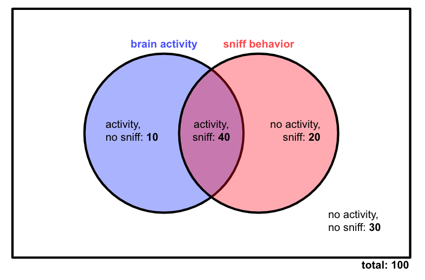
Our first question is: Are activity in this brain region and sniff behavior related?
First, let’s calculate \(p(A)\) (the probability of brain activity) and \(p(B)\) (the probability of sniff behavior) based on our data. That involves counting up the number of trials in which the event happens, and then dividing that number by the total number of trials.
Let’s also calculate the probability of the complements of these events — that is, the probability that they don’t happen. We express the complement of an event \(K\) as \(p(K')\) or \(p(!K).\)
These calculations allow us to observe something really important: \(p(A) + p(!A) = 1,\) and \(p(B) + p(!B) = 1.\) This should make sense: If we take all the elements of our sample space where a particular event happens, and all the elements where it doesn’t happen, that should cover our entire sample space.
Probability Rule
The probability of an event \(K\) and its complement \(!K\) always sum to 1.
Let’s calculate a few more probabilities from this experiment. What’s the probability that both the mouse sniffs and the brain region is active, \(p(A,B)\)? Well, to calculate that, we just divide the number of trials where both events happen by the total number of trials.
This quantity is known as the joint probability of \(A\) and \(B\). Note that it’s less than both \(p(A)\) and \(p(B)\), which makes sense — for a trial to count as part of the event \(A,B\), it must also count toward both \(A\) and \(B\) individually. In our Venn diagram, we are looking at the purple intersection in the middle, which is smaller than each circle.
Definition
The joint probability of two events \(J\) and \(K\), \(p(J,K)\), is the probability that they both occur. It must be less than or equal to the probabilities of the individual events, \(p(J)\) and \(p(K)\).
Next, let’s calculate the probability of \(A\) given that \(B\) happened, which we write as \(P(A|B)\). That is, we restrict our sample space to only those trials where the mouse did sniff. Then we say, given the mouse sniffed, how likely is it that the neurons also fired? Since we are changing our sample space, the denominator of our calculation is going to change — from the total number of trials, 100, to the total number of trials in which the mouse sniffed, 60.
And we can do the same to calculate the probability that the mouse sniffed given that the brain region was active:
Definition
The conditional probability of an event \(J\), conditioned on another event \(K\) — or \(p(J|K)\) — is the probability that \(J\) occurred, under the assumption that \(K\) occurred.
So, to review, we have calculated the following probabilities:
We can use these probabilities to demonstrate a really important identity. Let’s say we know \(p(B|A)\) and \(p(A)\) — that is, the probability that the brain region was active, and the probability that the mouse sniffed given that the brain region was active. Can we use these quantities to calculate the joint probability \(p(A,B)\) — that is, the probability that both events happened? Yes! We just have to take \(p(B|A)p(A)\).
Why does this work? Well, let’s look at how we calculated \(p(B|A)\) and \(p(A)\):
Note that this same logic works in the other direction, so we can also say \(p(A,B) = p(A|B)p(B).\)
We can test this using the numbers we calculated above!
Probability Rule
The joint probability of two events, \(J\) and \(K\), is the product of the probability of one of those events and the probability of the second event conditioned on the first event.
We’ve done lots of useful calculations so far, but we haven’t yet answered our original question — is brain activity in this region related to sniffing behavior? In other words, we want to know whether or not brain activity and sniffing are independent. If brain activity and sniffing behavior are not related, then whether one of them happens should not affect the chances of the other one happening.
Exercise
If sniffing and brain activity are independent, what should our Venn diagram look like? Assume that the probability of the mouse sniffing is still 0.6, and the probability of brain activity is still 0.5.
Solution
Since the probability of sniffing is 0.6, we expect that the mouse will sniff on 60 trials. On how many of those trials will the neurons also fire? Since we have assumed that sniffing and brain activity are independent, we should expect to see brain activity on half of the sniffing trials — 30 of those trials — because whether or not the mouse sniffed shouldn’t affect the probability of brain activity.
That leaves 30 sniffing, no activity trials. We also know that there should be 50 brain activity trials total, so we would expect 20 trials with activity but no sniffing. Here’s what the complete Venn diagram would look like:
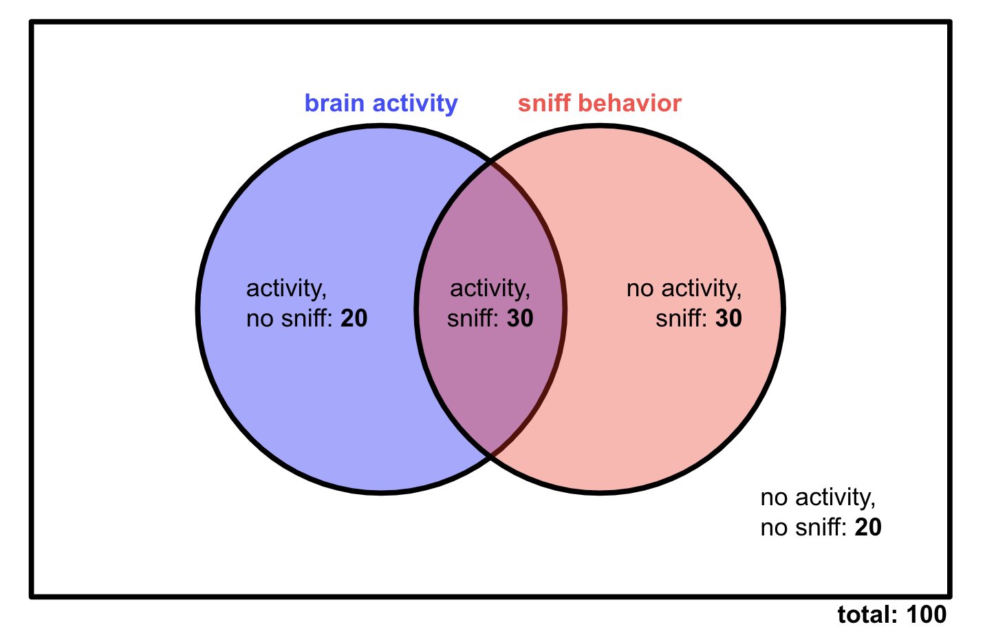
This isn’t what we observed in our data! So sniffing and brain activity are not independent in our experiment — the two events are connected, at least statistically speaking.
If brain activity and sniffing are independent, then \(p(A|B) = p(A)\) — whether or not the mouse sniffed has no effect on the probability of brain activity. The opposite is also true: \(p(B|A) = p(B).\) This yields an important identity:
So if two events are independent, their joint probability is just the product of their probabilities. We can see this using the Venn diagram from the previous exercise:
Probability Rule
If two events \(J\) and \(K\) are independent — that is, the fact that one happened has no effect on the probability of the other — you can calculate their joint probability by multiplying their individual probabilities.
Independence is NOT the same as mutual exclusivity
A very common mistake is to assume that independence is equivalent to mutual exclusivity, which means that two events never happen at the same time. In fact, the two are very different. For two events \(J\) and \(K\) to be mutually exclusive, we must have \(p(J,K) = 0.\) But looking at the previous probability rule, we can see that this will only happen for independent events \(J\) and \(K\) if the probability of at least one of them is already 0.
The difference between mutual exclusivity and independence makes sense if we think about our mouse experiment. If the mouse never sniffed when the brain region was active, we would probably assume that the brain region somehow inhibited sniffing behavior! That certainly wouldn’t make those two events independent.
We have one last important probability rule to cover. We know how to find the probability that our events \(A\) and \(B\) both happen — that’s just \(p(A,B).\) But what about the probability that either event happens — that the mouse sniffs, or the brain region is active, or both? We can really easily calculate this probability, which we write as \(p(A \cup B),\) from our Venn diagram:
How do I calculate this probability? Naïvely, we might think that we should just add \(p(A)\) and \(p(B)\):
Ok, that doesn’t quite work. The issue here is that we have essentially added everything in the red circle, and everything in the blue circle. But both circles contain that purple overlap — which means we have counted the purple overlap, or \(p(A,B),\) twice. So the trick is to add the probabilities of \(A\) and \(B\), but then to subtract their joint probability:
Probability Rule
To add the probabilities of two events, \(J\) and \(K\), add the probabilities of the events individually and then subtract their joint probability.
Probability Distributions#
Random Variables#
We’ve been focusing so far on 100 trials worth of data that we have already collected. But let’s say we keep running our experiment. What can we say about the 101st trial? Well, based on what we’ve already seen, we can estimate:
We can represent these facts graphically:

The \(y\)-axis here represents, of course, the probability of the different events. But what’s the \(x\)-axis? Formally speaking, the \(x\)-axis represents the random variable \(X\), which can take on four different values — \(A,B\), \(A,!B\), \(!A,B\), \(!A,!B\).
Definition
An random variable is a variable that represents the outcome of a probabilistic process. Random variables are typically written as capital letters.
Warning
Technically speaking, random variables should have numerical values. So to make the random variable \(X\) really work, we have to assign some values to our outcomes — like \(A,B = 0,\) \(A,!B = 1\), \(!A,B = 2,\) \(!A,!B = 3.\) In most cases, assigning values to outcomes isn’t quite so arbitrary. For example, a random variable might count the number of heads in 10 coin tosses.
With the language of random variables, we can rewrite the outcome probabilities for the 101st trial a bit more formally:
In this new formalism, \(p\) isn’t just a cue telling us to take the probability of some event — it’s a function of the random variable \(X.\) In particular, it is the probability distribution of \(X.\)
Definition
A probability distribution is a function that maps the set of possible values of a random variable to their probabilities.
The function \(p(X)\) may also be referred to as the probability mass function, if \(X\) takes on discrete values.
Since a random variable must always take on some value, but cannot take on two values at once, a probability distribution must always sum to 1.
In the rest of this section, we are going to learn about some useful probability distributions, as well as some important features of random variables.
The Binomial Distribution#
For the rest of this lesson, we are going to forget about behavior and focus on neuron activity. Let’s say that a neuron has a 0.6 probability of spiking. We represent the spiking state as 1, and the rest state as 0, and we use the random variable \(X\) to capture the neuron’s state at a given point in time. So we have
We can easily represent this graphically:

Our probability distribution \(p(X)\) here is called the Bernoulli distribution.
Definition
The Bernoulli distribution describes the behavior of any random variable \(X\) with only two possible outcomes, 0 and 1. If the probability of one of those outcomes, \(p(X=1),\) is \(p\), then the Bernoulli distribution has the following probability mass function:
Exercise
Demonstrate that the algebraic description of the Bernoulli distribution above gives us the probabilities we expect for the possible values of \(X.\)
Solution
Plugging in the possible values for \(k\) — that is, 0 and 1 — we obtain
On its own, the Bernoulli distribution isn’t terribly interesting. But let’s extend it into something more useful. What happens when we combine two Bernoulli random variables? That is, what if we don’t look at a single neuron, but two similar neurons? If we use the random variable \(Y\) to capture the state of the second neuron, we get the following joint probabilities (assuming the neurons are independent):
Typically, when we are studying a population of similarly behaving neurons, we don’t care about the identity of each individual neuron. Instead, what we care about is the total number of neurons that are active or inactive. So let’s define a new random variable, \(N,\) that describes the number of neurons firing at a particular time. We have:

What if we look at 3 neurons at once? If the activity of the third neuron is represented using the random variable \(Z,\) we have:
We can again introduce a new random variable \(N\) to capture the number of neurons that fire:
All of these distributions \(p(N)\) are specific examples of what’s called the binomial distribution. The binomial distribution essentially collects a bunch of Bernoulli random variables and tells us the probability that some number of them will be equal to 1. The binomial distribution has two parameters — the probability \(p\) that any one of the Bernoulli random variables will be equal to 1, and \(n,\) the total number of Bernoulli random variables.
Let’s try to derive a general form for the probability mass function of a binomial distribution with parameters \(p\) and \(n.\) The question we need to answer is — if we have \(n\) Bernoulli variables with probability \(p,\) what’s the probability that exactly \(k\) of them will be equal to 1?
It’s easiest if we start by considering a specific sequence of the Bernoulli variables. That is, let’s find the probability that only the first \(k\) variables are all equal to 1. If that’s the case, the remaining \(n - k\) variables will all be 0. Since the variables are independent, we just have to multiply the probabilities of each of the first \(k\) variables being equal to 1 and of each of the last \(n-k\) being equal to 0:
But that’s not all we need. We don’t actually care about the order of the neurons — all we care about is the total number of active neurons. So we need to count the possible number of ways that \(k\) out of \(n\) neurons could be active. We won’t go into the details of why here, but that quantity, which we write \({n\choose k}\) (”\(n\) choose \(k\)”), is just
where \(!\) is the factorial, so
Combining these ingredients gives us our binomial probability density function.
Definition
The binomial distribution describes the probability that \(n\) independent Bernoulli random variables with probability \(p\) will have \(k\) successes. Its probability density function is:
If \(X\) is a binomially distributed random variable, we can write that using the following shorthand:
In general, the symbol \(\sim\) can be read “is drawn from”, e.g. “\(X\) is drawn from the binomial distribution with parameters \(n\) and \(p.\)
Exercise
You are studying a population of 10 neurons. The neurons are all independent, and they fire with probability 0.75. What is the probability that exactly 6 of the 10 neurons will fire?
Solution
In probability language, this question just asks us to find \(p(X=6),\) for \(X \sim B(10,0.75).\) Using the binomial probability density function, we have
Expected Value and Variance#
Here’s a question we might want to ask about a population of neurons — how many neurons do we expect to fire? Knowing the probability of any specific number of neurons firing is useful, but it doesn’t give us a specific prediction about how the population will behave.
What we are asking here, in probability language, is a question about the expected value of a random variable. We could potentially define this quantity in a variety of ways, but a sensible thing to do is to take a weighted average of the possible values of \(X\), where we weight each possible value \(X\) by its probability \(k.\)
Definition
The expected value of a random variable \(X\), or \(\mathbb{E}(X),\) is defined as the average of all the possible values of \(X,\) weighted by their probabilities. For a discrete random variable \(X,\) we can write
Exercise
Calculate the expected value of a a Bernoulli random variable with probability \(p\).
Solution
Remember, a Bernoulli random variable \(X\) can only take on two possible values. So all we have to do to execute our sum is to calculate \(k \times p(X=k)\) for both possible values of \(k.\)
So, what’s the answer to our original question — what’s the expected value of a binomial random variable? To calculate this expected value, we need to combine the definition of expected value and the probability density function for the binomial distribution.
To do this next step, we make a crucial observation: \(n - k = (n-1) - (k-1)\).
where \(j = k - 1.\) Looking back at the binomial probability density function, we can see that the probability density function for a binomial distribution \(B(n-1,p)\) is just \(\frac{n-1!}{k!(n-1) - k!} p^{k} (1-p)^{(n-1)-k}\).$ So the sum above is just the sum over a binomial probability density function. And the sum over the entirety of any probability distribution must be 1. So we can say
Thus, for \(X \sim B(n,p)\), we have \(\mathbb{E}(X) = np.\) In plain English, that means that, if we have \(n\) neurons that each fire with probability \(p,\) we should expect \(np\) of them to fire at any given time.
The expected value helps us the center of a probability distribution. But there’s another important feature of any distribution — how wide it is, or its spread. We describe its spread using a property called the variance. To calculate the variance of a distribution, we take a weighted average, just like for the expected value. But instead of taking a weighted average of the possible values of \(X\), we want a weighted average of \(X\)’s distance from the center of the distribution.
Definition
The variance of a random variable \(X\), or \(\mathbb{E}(X),\) is the the average of \((X - \mathbb{E}(X))^2\), weighted by \(p(X).\) In other words, it’s the weighted average of the squared distance from \(X\) to the center of the probability distribution.
Exercise
Calculate the variance of a a Bernoulli random variable with probability \(p\).
Solution
Just like when we calculated the expected value of a Bernoulli random variable \(X\), we solve this problem by considering the two possible values of \(X\)—0 and 1.
The Poisson Distribution#
Binomial distributions can be helpful for capturing the behavior of population of neurons. But what if we just want to focus on one neuron at a time? Is there a probability distribution that we can use to model how neurons fire?
In particular, let’s assume we are recording a series of spikes from a neuron. Instead of looking at each individual spike, we want to track the neuron’s firing rate over time. So we count up the number of times it spikes in every 10 millisecond window. Our results might end up looking something like this:
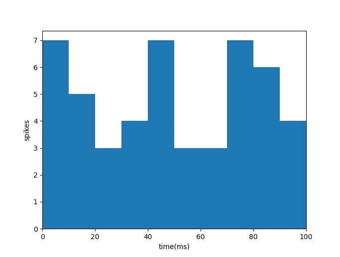
There’s obviously some randomness in how many times the neuron fires in each 10 ms window. And there’s a probability distribution that captures that randomness: the Poisson distribution. The Poisson distribution is designed to predict the number of times an event will happen in some time window. If the event’s occurrences are independent — that is, the fact that the event happened once, or twice, or three times has no effect on whether or not it will happen again — the Poisson distribution is the perfect model.
Warning
The firing rate plot above is not itself a Poisson distribution. The \(x\)-axis of a probability distribution is the random variable, and the \(y\)-axis is its probability. Instead, each bar in that plot represents a single sample from a Poisson distribution. To produce a firing-rate simulation using a Poisson distribution, you have to repeatedly sample from the distribution to get the firing rate in each time window.
Definition
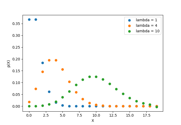
The Poisson distribution describes the probability that \(k\) independent events will occur within a particular time window. It has one parameter, \(\lambda.\) Its probability mass function is
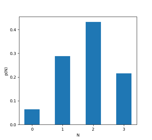
The below plot shows the Poisson probability mass function for several values of \(\lambda.\)
What’s the expected value of the Poisson distribution? Let’s calculate it. Just like with the binomial expected value, we’ll have to recall that any probability density function must sum to 1.
We won’t prove it here, but an interesting fact about the Poisson distribution is that its variance is also \(\lambda.\)
The Gaussian Distribution#
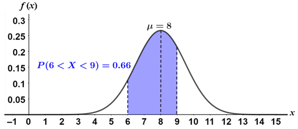
Thus far, we’ve been strictly dealing with discrete probability distributions — distributions for which \(X\) can only take on a finite number of values. But the probability distribution with which you are probably most familiar, the Gaussian distribution or normal distribution, is continuous. In fact, if \(X\) is normally distributed, it can take on any real value.
Because continuous random variables can take on an infinite number of values, the probability that \(p(X=k)\) for any specific value is 0 — if it were anything greater than 0, the total probability of \(X\) taking on any value would be infinite. So instead of defining a probability mass function to describe the distribution, we define a probability density function. We can then integrate that probability density function to find the probability that \(X\) will end up falling between any two values.
Okay, but why does this particular continuous distribution matter? We won’t get into the statistical details here, but it turns out that if you sample any random variable many times, the average of all of those observations is guaranteed to be a Gaussian random variable, as long as you make enough observations. To make that more concrete, if you observe 100 different neurons many many times, and average all of their firing rates, those average firing rate observations will follow a Gaussian distribution.
This makes the Gaussian distribution incredibly useful in biology, when we are often looking at the aggregate results of many simultaneous random processes — like the flip-flopping proteins and drifting neurotransmitters I mentioned in the introduction. If you are measuring some continuous variable in a biological experiment, and the value of that variable comes down to the aggregate behavior of many random processes, then it’s a good idea to model that variable using a Gaussian distribution.
Definition
The Gaussian distribution is a continuous probability distribution that describes the distribution of sample means for any random process. Its probability density function, expected value, and variance are:
Probabilistic Modeling#
We’ve spent all this time discussing probability distributions for one main reason: They are useful for modeling various phenomena in neuroscience. For example, we could define a random variable \(X\) to represent the intracellular voltage of a neuron, and we could draw values of \(X\) at any given time from a Gaussian distribution with mean \(\mu\) and standard deviation \(\sigma\):
Let’s say we want to model a specific neuron, from which we have intracellular recordings —that is, we have a bunch of data \(x_1, x_2, \cdots, x_n\) and we want to choose \(\mu\) and \(\sigma\) such that those \(x_i\) could have been believably drawn from that Gaussian distribution. How do we intelligently select \(\mu\) and \(\sigma\)? That’s the question that likelihood solves for us.
The Likelihood Function#
Our problem is this: We have some data \(\textbf{x}\) and a probabilistic model with a parameter \(\theta.\) We want to choose the parameter \(\theta\) that makes our data as likely as possible. In other words, we want to maximize \(p(\textbf{x} | \theta)\). That’s just a conditional probability. Essentially what we are doing is setting \(\theta\) to a bunch of different values, checking what the probability of our data \(\textbf{x}\) would be with all those different values of \(\theta\), and choosing the \(\theta\) that yields the highest probability.
\(p(\textbf{x}|\theta),\) where we hold \(\textbf{x}\) (the data we observed) fixed and let \(\theta\) vary, is called the likelihood of our data \(\textbf{x}.\) It can be a bit counterintuitive to have a conditional probability where we are conditioning on a parameter of a model. The trick is to think of the likelihood \(L(\theta)\) just like we would think of any other function. \(p(\textbf{x} | \theta)\) is going to have some algebraic form, and that algebraic form defines the likelihood function \(L(\theta).\)
Definition
The likelihood of a set of data under a particular model is the probability of observing those data, assuming that the model is true. A likelihood function is always a function of the model parameters; the data are fixed.
Let’s try an example. We observe \(A\) neurons, and \(a\) of them fire. What’s the likelihood of those data under a binomial distribution with probability parameter \(p\)?
To find the value of \(p\) for which a binomial distribution would be most likely to produce the data we observed, we would just have to maximize \({A\choose a}p^a(1-p)^{A-a}\) with respect to \(p\).
One important note — you may recall that probability density functions for continuous distributions don’t actually give us the probability of a random variable taking any particular value, since all such probabilities are 0. So if we are, say, dealing with a Gaussian, how would we determine the value of \(\mu\) or \(\sigma\) that maximizes the probability of some observation \(x_i\)?
Well, the probability of observing our data is always 0, so we can’t maximize that. So let’s be a little looser here. What’s the likelihood of making an observation at most \(\Delta x\) away from \(x\)?
If we assume \(\Delta X\) is very small, then the probability density function is constant within the range we are considering, so
\(\Delta x\) is a constant, so it has no effect on the values of \(\mu\) and \(\sigma\) that optimize this expression. So we can safely ignore it and just say
which has exactly the same form as our probability density function. So for continuous distributions, we can construct likelihoods exactly as we do for discrete distributions — by going directly to the probability density/mass function.
Exercise
What is the likelihood of making a single observation \(k\) under a Poisson distribution with parameter \(\lambda\)?
Solution
This likelihood is going to look exactly like our Poisson probability mass function. But remember, it is fundamentally different — \(k\) here is fixed, whereas \(\lambda\) is not.
Exercise
You want to find the likelihood of a large dataset with observations \(x_1, x_2, \cdots, x_n\) under a model that you are investigating. The likelihood of one observation under the model is \(L(x_i).\) What is the likelihood of all the observations? Assume the observations are independent.
Solution
The likelihood is just the probability (or probability density) of observing some data given a model. So we combine likelihoods just like we combine probabilities — if they are independent, we multiply them. So:
To maximize the likelihood, we have to differentiate it with respect to our parameter — \(\lambda\) for a Poisson distribution, \(p\) for a binomial distribution, etc — and set it to 0. That isn’t too hard as long as we have a small amount of data and our likelihood function is simple.
But what if we have a bunch of observations? The likelihood of each observation might have a fairly simple form — \(L(x_i)\) — but if we are looking at many observations, we have to take the product of the likelihoods of all the observations — \(L(x_1)\cdot L(x_2) \cdot \cdots \cdot L(x_n).\) Differentiating that extended product can get messy, fast. Is there anything we can do?
There is, as long as we remember our ultimate objective! All that we want to do with the likelihood function is maximize it. Let’s say our maximum occurs at the parameter value \(\theta_0.\) That means we have
for any \(\theta' \neq \theta_0.\) But what if we could find a function \(f(x)\) such that \(x_1 > x_2\) would imply \(f(x_1) > f(x_2)\)? Then we would have
In other words, \(f(L(x))\) would be maximized in exactly the same place as \(L(x)\) — at \(\theta_0.\) So maximizing \(f(L(x))\) would do just as good a job at helping us find our optimal parameter.
It turns out that any strictly increasing function satisfies our requirement for \(f\). And one strictly increasing function that helps us out here is the natural logarithm, \(\ln(x).\)
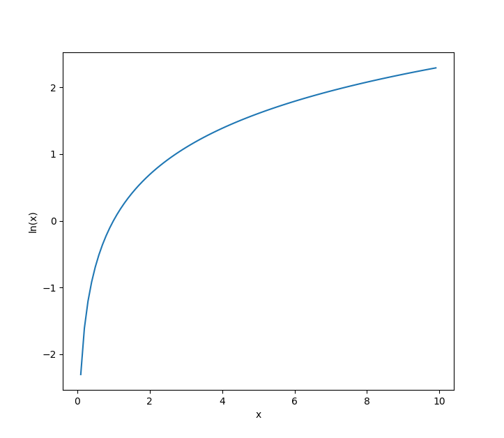
Why is \(\ln(x)\) so helpful here? Well, let’s see what happens when we apply it to our likelihood function for multiple observations!
I used the fact that \(\ln(a\cdot b) = \ln(a) + \ln(b)\) to turn our ugly product into a very manageable sum. Sums are super easy to differentiate — you just differentiate every element of the sum separately — so this new log likelihood is much easier to maximize than the original likelihood!
To wrap up, let’s apply all of these ideas! Let’s say you observe a series of discrete events over a period of \(n\) seconds — say, neuron spikes — and you want to model them using a Poisson distribution. You count the number of events that occur over your chosen time windows, and you obtain a series of spike counts \(k_1, k_2, \cdots, k_n.\) What parameter \(\lambda\) should we use to build a Poisson distribution that best models this neuron?
We start by calculating the likelihood.
Maximizing a product this big is tricky. So let’s try to maximie the log likelihood (which I will denote \(LL(x)\)) instead.
Now, let’s maximize the log likelihood by differentiating it with respect to \(\lambda\) and setting that derivative to 0!
So, \(\lambda\) should just be the average of all the \(k_i\)! That makes a lot of intuitive sense — remember, \(\lambda\) is the expected value of the Poisson distribution.